Covid-19 forecasting
Table of Contents
Introduction#
This is the third part of our series about Covid19 data analysis. This series is inspired after the proposed Kaggle challenge. This notebook introduces some practical examples of univariate time series forecasting.
We introduces the Python statsmodel module which provides a set of statistical tools for conducting statistical tests and data exploration. We focus on the time series analysis module offered in this package to run basic time series forecasting predicting the evolution of cases in the Covid19 pandemia.
Assumptions
- You succesfully run the Covid19 visualization notebook
- You have an already running Jupyter environment
- You are familiar with Pandas
- You have heard about Matplotlib
- The covid19 files are available in the path covid19-global-forecasting-week-2
Load the data#
Load the CSV data using pandas. In this case, we use the read_csv function indicating the date parser to be used. Working with dates is going to be particularly useful when working with time series.
import pandas as pd
import datetime
data = pd.read_csv('covid19-global-forecasting-week-2/train.csv',parse_dates=['Date'],
                   date_parser=lambda x: datetime.datetime.strptime(x, '%Y-%m-%d'))
data
| Id | Country_Region | Province_State | Date | ConfirmedCases | Fatalities | |
|---|---|---|---|---|---|---|
| 0 | 1 | Afghanistan | NaN | 2020-01-22 | 0.0 | 0.0 |
| 1 | 2 | Afghanistan | NaN | 2020-01-23 | 0.0 | 0.0 |
| 2 | 3 | Afghanistan | NaN | 2020-01-24 | 0.0 | 0.0 |
| 3 | 4 | Afghanistan | NaN | 2020-01-25 | 0.0 | 0.0 |
| 4 | 5 | Afghanistan | NaN | 2020-01-26 | 0.0 | 0.0 |
| ... | ... | ... | ... | ... | ... | ... |
| 18811 | 29360 | Zimbabwe | NaN | 2020-03-21 | 3.0 | 0.0 |
| 18812 | 29361 | Zimbabwe | NaN | 2020-03-22 | 3.0 | 0.0 |
| 18813 | 29362 | Zimbabwe | NaN | 2020-03-23 | 3.0 | 1.0 |
| 18814 | 29363 | Zimbabwe | NaN | 2020-03-24 | 3.0 | 1.0 |
| 18815 | 29364 | Zimbabwe | NaN | 2020-03-25 | 3.0 | 1.0 |
18816 rows × 6 columns
China was the origin of Covid19. Its curve of infection is the longest one among the curves available in the dataset. We are going to get a sample filtering all the data corresponding to China. Remember that in the case of China we have information about the evolution for every province. In order, to work with an aggregated value per country and day, we have to aggregate the data. Check the previous notebooks for more details about this operation.
china = data.where(data.Country_Region=='China').groupby(['Date'],as_index=False).sum()
china
| Date | Id | ConfirmedCases | Fatalities | |
|---|---|---|---|---|
| 0 | 2020-01-22 | 214533.0 | 548.0 | 17.0 |
| 1 | 2020-01-23 | 214566.0 | 643.0 | 18.0 |
| 2 | 2020-01-24 | 214599.0 | 920.0 | 26.0 |
| 3 | 2020-01-25 | 214632.0 | 1406.0 | 42.0 |
| 4 | 2020-01-26 | 214665.0 | 2075.0 | 56.0 |
| ... | ... | ... | ... | ... |
| 59 | 2020-03-21 | 216480.0 | 81305.0 | 3259.0 |
| 60 | 2020-03-22 | 216513.0 | 81435.0 | 3274.0 |
| 61 | 2020-03-23 | 216546.0 | 81498.0 | 3274.0 |
| 62 | 2020-03-24 | 216579.0 | 81591.0 | 3281.0 |
| 63 | 2020-03-25 | 216612.0 | 81661.0 | 3285.0 |
64 rows × 4 columns
import matplotlib.pyplot as pyplot
fig = pyplot.figure(figsize=(10,5))
ax1 = fig.add_subplot()
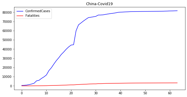
china.ConfirmedCases.plot(ax=ax1,color='blue',legend=True, title='China-Covid19')
china.Fatalities.plot(ax=ax1,color='red',legend=True)
pyplot.show()
Univariate time series analysis#
The plot above shows the evolution of confirmed cases and fatalities for China during the Covid19 crisis. This seems the common profile of any pandemic. First, the number of cases increases until it reaches a plateau. Then, it stays stable until the cases decrease with an increment in the number of fatalities.
One of the most important problems to be resolved in this case, like in any other time series is: can we forecast the number of new cases and/or fatalities with some accuracy?
We start working with the China time series. Before starting we need to make some preparation to work with datetime indices. These are common operations in Pandas. We remove the Id column and convert the Date column into our new row index. Additionally, we set the frequency of the index to days by executing china.index.freq='d'. This is particularly helpful when using Pandas time series.
china = china.set_index('Date')
china.drop(['Id'], axis=1, inplace=True)
# The index is a time series with a frequency of days
china.index.freq='d'
Simple exponential smoothing#
If we try to predict any future value in an univariate time series, the first thing we have to consider is the fact that future observations depend on past and present observations. If $\hat{y}t$ is the forecast of variable $x$ at time $t$ and $\hat{y}{t+h|t}$ the forecast of variable $x$ at time $t+h$ given time $t$, a forecast equation could be something like this.
$$ \begin{align} \hat{y}_{t+h|t} = l_t \end{align} $$
Which basically means that our predictions at time $t+h$ given observations at time $t$ are the result of a function $l$ at time $t$. And what is this function? We are going to use a simple exponential smoothing (SES) function.
$$ \begin{align} l_1 &= \alpha y_1 + (1- \alpha) l_{0} \end{align} $$
Which is a formal way of saying that the current value depends on the previous value multiplied by a smoothing factor $ \alpha $. If we continue developing the equation we have
$$ \begin{align*} l_1 &=\alpha y_1 + (1-\alpha) l_{0} \ l_2 &=\alpha y_2 + (1-\alpha) l_{1} = \alpha y_2 + \alpha(1-\alpha) y_1 + (1-\alpha)^2 l_{0} \ l_3 &=\alpha y_3 + (1-\alpha) l_{2} = \sum_{j=0}^{2}\alpha(1-\alpha)^jy_{3-j}+(1-\alpha)^3l_{0} \ \vdots \ l_t &= \sum_{j=0}^{t-1}\alpha(1-\alpha)^j y_{t-j}+(1-\alpha)^tl_0 \end{align*} $$
Therefore, the forecasting equation is:
$$ \begin{align*} \hat{y}{t+h|t} &= \sum{j=1}^{t}\alpha(1-\alpha)^{t-j} y_{j}+(1-\alpha)^tl_0 \end{align*} $$
The $\alpha$ value should be chosen to minimize the mean squared error (MSE)
$$ \begin{align*} MSE = \frac{1}{T} \sum_{t=1}^{T} (y_t+\hat{y}_{t|t-1})^2 \end{align*} $$
There is no closed solution to find $\alpha$. Least squares can be a simple and valid method to set the value.
We are going to use the implementation available at the statsmodels library to make some predictions for the number of confirmed cases in China starting at 2020-03-20.
from statsmodels.tsa.holtwinters import SimpleExpSmoothing
# We previously set dates as the row index. Now we can use indexes to select rows.
china_train = china[:'2020-03-20']
china_test = china['2020-03-21':]

# Chose a model for confirmed cases
model = SimpleExpSmoothing(china_train.ConfirmedCases)
# Fit the model for the given observations
model_fit = model.fit()
We have fit a model using SES and the number of confirmed cases. It is extremely useful to check what are the params for this model and understand how well our fitting process did.
# Check the params for the model
display(model_fit.params)
# Lets observe a summary about the fitting
model_fit.summary()
{'smoothing_level': 1.0,
 'smoothing_slope': nan,
 'smoothing_seasonal': nan,
 'damping_slope': nan,
 'initial_level': 548.0,
 'initial_slope': nan,
 'initial_seasons': array([], dtype=float64),
 'use_boxcox': False,
 'lamda': None,
 'remove_bias': False}
| Dep. Variable: | endog | No. Observations: | 59 |
|---|---|---|---|
| Model: | SimpleExpSmoothing | SSE | 421717800.000 |
| Optimized: | True | AIC | 935.156 |
| Trend: | None | BIC | 939.311 |
| Seasonal: | None | AICC | 935.897 |
| Seasonal Periods: | None | Date: | Fri, 03 Apr 2020 |
| Box-Cox: | False | Time: | 20:51:35 |
| Box-Cox Coeff.: | None |
| coeff | code | optimized | |
|---|---|---|---|
| smoothing_level | 1.0000000 | alpha | True |
| initial_level | 548.00000 | l.0 | True |
We can set the $\alpha$ parameter by setting the smoothing_level value in the model.fit call. However, if we do not set any value, the library will find it for us. In this case $\alpha$ was automatically set to 1 with $l_0=548$ (initial_level in the summary table).
Now we are going to fit some models manually setting the $\alpha$ parameter and compare the obtained output.
import matplotlib.pyplot
# Fit with some alphas
fit025 = model.fit(smoothing_level=0.25)
fit05 = model.fit(smoothing_level=0.5)
fit075 = model.fit(smoothing_level=0.75)

ax = china_train.ConfirmedCases.plot(color='black', legend=True)
model_fit.fittedvalues.plot(ax=ax, color='blue', style='--', legend=True, label=r'Auto $\alpha=%s$'%model_fit.params['smoothing_level'])
fit025.fittedvalues.plot(ax=ax, color='red', style='--', legend=True, label=r'$\alpha=0.25$' )
fit05.fittedvalues.plot(ax=ax, color='green', style='--', legend=True, label=r'$\alpha=0.5$')
fit075.fittedvalues.plot(ax=ax, color='grey', style='--', legend=True, label=r'$\alpha=0.75$' )

pyplot.show()
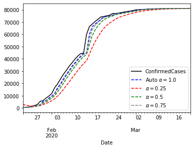
The plot above shows that $\alpha=1$ gives the best approximation to the curve. Now that we know that $\alpha=1$ brings the best performance, we can think about forecasting with that model.
# Lets make some predictions
predicted = model_fit.predict(start='2020-03-21',end='2020-03-25').rename('Predicted ConfirmedCases')
ax = china_train.ConfirmedCases.plot(color='black', legend=True)
china_test.ConfirmedCases.plot(ax = ax, color='blue', legend=False)
predicted.plot(ax=ax, color='blue', style='--', legend=True)
pyplot.show()
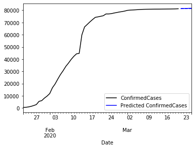
The plot the whole time series and a five days prediction. We better use some zoom.
ax = china_train.ConfirmedCases['2020-03-15':'2020-03-25'].plot(color='black',legend=True)
china_test.ConfirmedCases.plot(ax = ax, color='blue', legend=True, label='ConfirmedCases to predict')
predicted.plot(ax=ax, color='blue', style='--', legend=True)
pyplot.show()
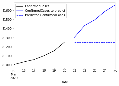
Observe that the iterative prediction always returns the same value. This is because this function is a flat forecast function. There is no trend, seasonality or other value that can make this prediction to evolve. So finally, what we have is the mean of a future:
$$ \begin{align*} \hat{y}{T+h|T} = \hat{y}{T+1|T}, \space h=2,3,… \end{align*} $$
Holt-Winters#
The flat nature of multiple steps forecasting of SES is not a good solution if we need a prediction at $T+h$. However, there are other approaches which basically include additional elemnts such as seasonality or trend. For example, the Holt’s local trend method adds a $\beta^*$ factor that controls the trend:
$$ \begin{align*} Forecast: && \hat{y}{t+h|t} &= l_t + hb_t \ Level: && l_t &= \alpha y_t + (1-\alpha)(l{t-1}+b_{t-1}) \ Trend: && b_t &= \beta^(l_t-l_{t-1})+(1-\beta^)b_{t-1} \end{align*} $$
In this approach, $l_t$ estimates the level while $bt$ estimates the slope. The extension of the formula requires to estimate $\alpha$, $\beta=\alpha\beta^*$,$l_0$ and $b_0$.
Let’s compare the forecast obtained from Holt-Winters for the previous scenario.
from statsmodels.tsa.holtwinters import Holt

# Fit a Holt-Winters model
holt_model = Holt(china_train.ConfirmedCases)
holt_fitted = holt_model.fit()
holt_fitted.summary()
| Dep. Variable: | endog | No. Observations: | 59 |
|---|---|---|---|
| Model: | Holt | SSE | 243476583.261 |
| Optimized: | True | AIC | 906.747 |
| Trend: | Additive | BIC | 915.057 |
| Seasonal: | None | AICC | 908.362 |
| Seasonal Periods: | None | Date: | Fri, 03 Apr 2020 |
| Box-Cox: | False | Time: | 20:51:36 |
| Box-Cox Coeff.: | None |
| coeff | code | optimized | |
|---|---|---|---|
| smoothing_level | 1.0000000 | alpha | True |
| smoothing_slope | 0.2715660 | beta | True |
| initial_level | 398.89608 | l.0 | True |
| initial_slope | 657.75311 | b.0 | True |
holt_predicted = holt_fitted.predict(start='2020-03-21', end='2020-03-25').rename('Predicted ConfirmedCases')

fig = pyplot.figure(figsize=(15,10))
ax1 = fig.add_subplot(2,2,1)
china_train.ConfirmedCases['2020-03-15':'2020-03-25'].plot(ax=ax1,color='black',legend=True,
                                                           title='Simple Exponential Smoothing Excerpt')
china_test.ConfirmedCases.plot(ax = ax1, color='blue', legend=True, label='ConfirmedCases to predict')
predicted.plot(ax=ax1, color='blue', style='--', legend=True)

ax2 = fig.add_subplot(2,2,2)
china_train.ConfirmedCases['2020-03-15':'2020-03-25'].plot(ax=ax2, color='black',legend=True,
                                                           title='Holt Winters Excerpt')
china_test.ConfirmedCases.plot(ax = ax2, color='blue', legend=True, label='ConfirmedCases to predict')
holt_predicted.plot(ax=ax2, color='blue', style='--', legend=True)

ax4 = fig.add_subplot(2,2,3)
china_train.ConfirmedCases.plot(ax=ax4, color='black',legend=True, title='Simple Exponential Smoothing')
model_fit.fittedvalues.plot(ax=ax4, color='blue', style='--', legend=True, label='Predicted ConfirmedCases')

ax3 = fig.add_subplot(2,2,4)
china_train.ConfirmedCases.plot(ax=ax3, color='black',legend=True, title='Holt Winters')
holt_fitted.fittedvalues.plot(ax=ax3, color='blue', style='--', legend=True, label='Predicted ConfirmedCases')

pyplot.tight_layout()
pyplot.show()
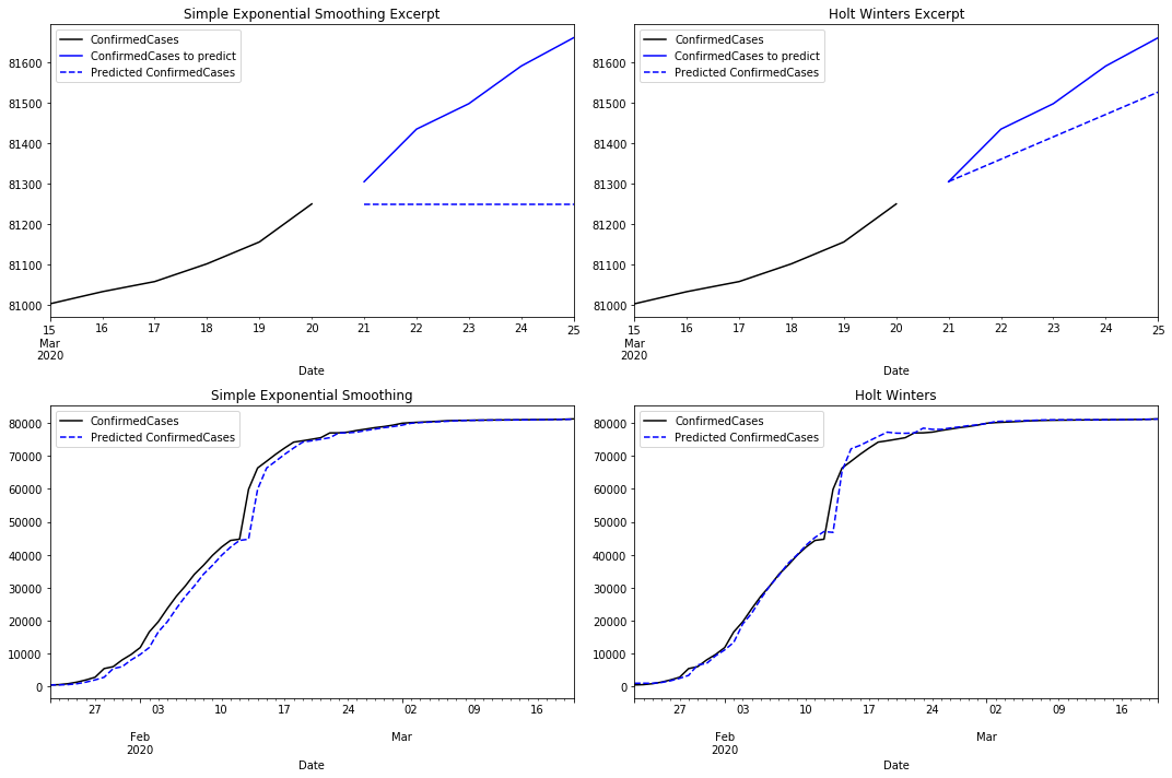
Comparing SES with the Holt Winters predictions there are clear differences. As we mentioned before, the prediction for the next five days is flat in the first case. Holt Winters uses its trend component to predict an increment in the number of cases.
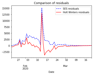
When comparing how both models fit the time series, SES reacts with some latency returning an approximation with some lag. Holt Winters reacts earlier by capturing the trend. However, it reacts with some latency when the trend changes. If we compare the residuals for both models we notice that Holt Winters performs better than SES.
ax=model_fit.resid.plot(color='blue', style='--', legend=True, label='SES residuals', title='Comparison of residuals')
holt_fitted.resid.plot(ax=ax, color='red', legend=True, label='Holt Winters residuals')
pyplot.show()
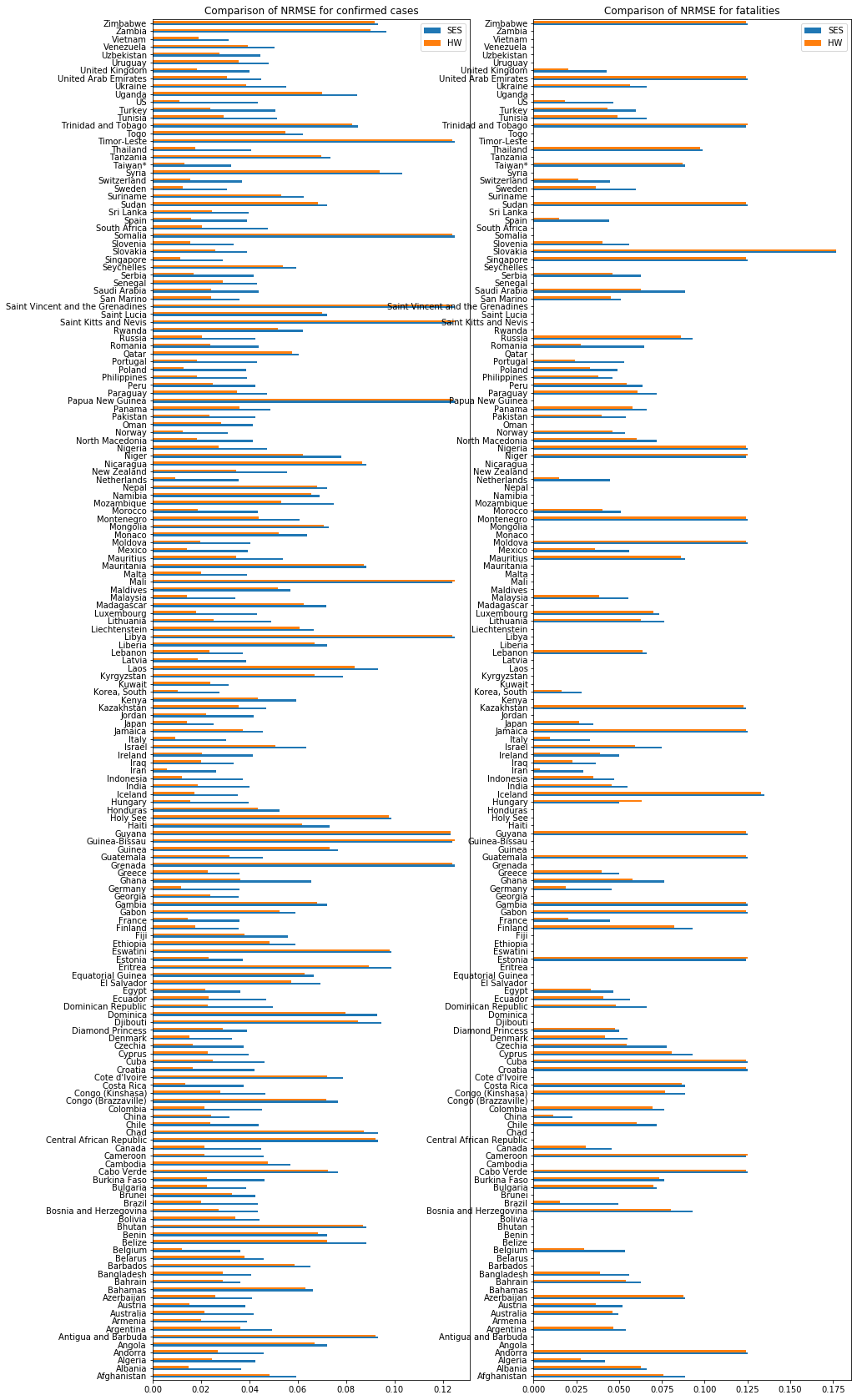
At the moment of writing this notebook the most complete Covid-19 time series corresponds to China. However, we can check the quality of the fitting models for every country in the dataset. We can expect that any Holt Winters model will return better predictions than SES. For the sake of exhaustiveness we compare the performance of SES and Holt Winters predicting the number of confirmed cases and fatilities for every country in the dataset. The range of observed values for every country in the dataset may dramatically vary. This makes useless the comparison of RMSE values. We employ the Normalized Squared Error (NRMSE) which normalizes the RMSE using the max and min observed values. This is, $\mathit{NRMSE} = \frac{\mathit{RMSE}}{y_{max}-y_{min}}$.
Note: Observations may dramatically vary between countries. We ignore countries with no fatalities nor confirmed cases.
# Accumulate observations per country and date. This is required to aggregate observations for multiple provinces
# in the same country.
data=data.groupby(['Country_Region','Date'],as_index=False,).sum()
display(data)
| Country_Region | Date | Id | ConfirmedCases | Fatalities | |
|---|---|---|---|---|---|
| 0 | Afghanistan | 2020-01-22 | 1 | 0.0 | 0.0 |
| 1 | Afghanistan | 2020-01-23 | 2 | 0.0 | 0.0 |
| 2 | Afghanistan | 2020-01-24 | 3 | 0.0 | 0.0 |
| 3 | Afghanistan | 2020-01-25 | 4 | 0.0 | 0.0 |
| 4 | Afghanistan | 2020-01-26 | 5 | 0.0 | 0.0 |
| ... | ... | ... | ... | ... | ... |
| 11067 | Zimbabwe | 2020-03-21 | 29360 | 3.0 | 0.0 |
| 11068 | Zimbabwe | 2020-03-22 | 29361 | 3.0 | 0.0 |
| 11069 | Zimbabwe | 2020-03-23 | 29362 | 3.0 | 1.0 |
| 11070 | Zimbabwe | 2020-03-24 | 29363 | 3.0 | 1.0 |
| 11071 | Zimbabwe | 2020-03-25 | 29364 | 3.0 | 1.0 |
11072 rows × 5 columns
import numpy as np


def computeErrors(ymax,ymin,fitted):
    '''
    Compute the normalized RMSE for this model
    $$
    \mathit{NRMSE} = \frac{\mathit{RMSE}}{y_{max}-y_{min}}
    $$
    '''
    RMSE = np.sqrt(np.sum(np.power(fitted.resid,2))/len(fitted.resid))
    NRMSE = RMSE / (ymax-ymin)
    return NRMSE

# Fit a model for every country

# Get the list of all the available countries
countries = data.Country_Region.unique()


nrmse = pd.DataFrame(columns=['SES-Confirmed','SES-Fatalities','HoltWinters-Confirmed','HoltWinters-Fatalities'],
                    index=countries)

# Because we are blindly computing a large number of models, some of them may result in convergence problems.
# We ignore them.
import warnings
warnings.filterwarnings('ignore')

for country in countries:
    excerpt = data[data.Country_Region==country]
    maxConfirmed = excerpt.ConfirmedCases.max()
    minConfirmed = excerpt.ConfirmedCases.min()
    maxFatalities = excerpt.Fatalities.max()
    minFatalities = excerpt.Fatalities.min()
    # Skip it if we have no relevant data
    if maxConfirmed == 0 or maxFatalities==0:
        print('%s skipped because there is no relevant data'%(country))
        next
    else:
        print('%s processing'%(country))

    # Models with ses
    ses_confirmed = SimpleExpSmoothing(excerpt.ConfirmedCases)
    ses_fatalities = SimpleExpSmoothing(excerpt.Fatalities)
    # Models with Holt Winters
    hw_confirmed = Holt(excerpt.ConfirmedCases)
    hw_fatalities = Holt(excerpt.Fatalities)

    # Fit models
    ses_confirmed_fit = ses_confirmed.fit()
    ses_fatalities_fit = ses_fatalities.fit()
    hw_confirmed_fit = hw_confirmed.fit()
    hw_fatalities_fit = hw_fatalities.fit()

    # Fill our dataframe
    nrmse.loc[country]={
        'SES-Confirmed': computeErrors(maxConfirmed,minConfirmed,ses_confirmed_fit),
        'SES-Fatalities': computeErrors(maxFatalities,minFatalities,ses_fatalities_fit),
        'HoltWinters-Confirmed': computeErrors(maxConfirmed,minConfirmed,hw_confirmed_fit),
        'HoltWinters-Fatalities': computeErrors(maxFatalities,minFatalities,hw_fatalities_fit)
    }

nrmse
Afghanistan processing
Albania processing
Algeria processing
Andorra processing
Angola skipped because there is no relevant data
Antigua and Barbuda skipped because there is no relevant data
Argentina processing
Armenia skipped because there is no relevant data
Australia processing
Austria processing
Azerbaijan processing
Bahamas skipped because there is no relevant data
Bahrain processing
Bangladesh processing
Barbados skipped because there is no relevant data
Belarus skipped because there is no relevant data
Belgium processing
Belize skipped because there is no relevant data
Benin skipped because there is no relevant data
Bhutan skipped because there is no relevant data
Bolivia skipped because there is no relevant data
Bosnia and Herzegovina processing
Brazil processing
Brunei skipped because there is no relevant data
Bulgaria processing
Burkina Faso processing
Cabo Verde processing
Cambodia skipped because there is no relevant data
Cameroon processing
Canada processing
Central African Republic skipped because there is no relevant data
Chad skipped because there is no relevant data
Chile processing
China processing
Colombia processing
Congo (Brazzaville) skipped because there is no relevant data
Congo (Kinshasa) processing
Costa Rica processing
Cote d'Ivoire skipped because there is no relevant data
Croatia processing
Cuba processing
Cyprus processing
Czechia processing
Denmark processing
Diamond Princess processing
Djibouti skipped because there is no relevant data
Dominica skipped because there is no relevant data
Dominican Republic processing
Ecuador processing
Egypt processing
El Salvador skipped because there is no relevant data
Equatorial Guinea skipped because there is no relevant data
Eritrea skipped because there is no relevant data
Estonia processing
Eswatini skipped because there is no relevant data
Ethiopia skipped because there is no relevant data
Fiji skipped because there is no relevant data
Finland processing
France processing
Gabon processing
Gambia processing
Georgia skipped because there is no relevant data
Germany processing
Ghana processing
Greece processing
Grenada skipped because there is no relevant data
Guatemala processing
Guinea skipped because there is no relevant data
Guinea-Bissau skipped because there is no relevant data
Guyana processing
Haiti skipped because there is no relevant data
Holy See skipped because there is no relevant data
Honduras skipped because there is no relevant data
Hungary processing
Iceland processing
India processing
Indonesia processing
Iran processing
Iraq processing
Ireland processing
Israel processing
Italy processing
Jamaica processing
Japan processing
Jordan skipped because there is no relevant data
Kazakhstan processing
Kenya skipped because there is no relevant data
Korea, South processing
Kuwait skipped because there is no relevant data
Kyrgyzstan skipped because there is no relevant data
Laos skipped because there is no relevant data
Latvia skipped because there is no relevant data
Lebanon processing
Liberia skipped because there is no relevant data
Libya skipped because there is no relevant data
Liechtenstein skipped because there is no relevant data
Lithuania processing
Luxembourg processing
Madagascar skipped because there is no relevant data
Malaysia processing
Maldives skipped because there is no relevant data
Mali skipped because there is no relevant data
Malta skipped because there is no relevant data
Mauritania skipped because there is no relevant data
Mauritius processing
Mexico processing
Moldova processing
Monaco skipped because there is no relevant data
Mongolia skipped because there is no relevant data
Montenegro processing
Morocco processing
Mozambique skipped because there is no relevant data
Namibia skipped because there is no relevant data
Nepal skipped because there is no relevant data
Netherlands processing
New Zealand skipped because there is no relevant data
Nicaragua skipped because there is no relevant data
Niger processing
Nigeria processing
North Macedonia processing
Norway processing
Oman skipped because there is no relevant data
Pakistan processing
Panama processing
Papua New Guinea skipped because there is no relevant data
Paraguay processing
Peru processing
Philippines processing
Poland processing
Portugal processing
Qatar skipped because there is no relevant data
Romania processing
Russia processing
Rwanda skipped because there is no relevant data
Saint Kitts and Nevis skipped because there is no relevant data
Saint Lucia skipped because there is no relevant data
Saint Vincent and the Grenadines skipped because there is no relevant data
San Marino processing
Saudi Arabia processing
Senegal skipped because there is no relevant data
Serbia processing
Seychelles skipped because there is no relevant data
Singapore processing
Slovakia processing
Slovenia processing
Somalia skipped because there is no relevant data
South Africa skipped because there is no relevant data
Spain processing
Sri Lanka skipped because there is no relevant data
Sudan processing
Suriname skipped because there is no relevant data
Sweden processing
Switzerland processing
Syria skipped because there is no relevant data
Taiwan* processing
Tanzania skipped because there is no relevant data
Thailand processing
Timor-Leste skipped because there is no relevant data
Togo skipped because there is no relevant data
Trinidad and Tobago processing
Tunisia processing
Turkey processing
US processing
Uganda skipped because there is no relevant data
Ukraine processing
United Arab Emirates processing
United Kingdom processing
Uruguay skipped because there is no relevant data
Uzbekistan skipped because there is no relevant data
Venezuela skipped because there is no relevant data
Vietnam skipped because there is no relevant data
Zambia skipped because there is no relevant data
Zimbabwe processing
| SES-Confirmed | SES-Fatalities | HoltWinters-Confirmed | HoltWinters-Fatalities | |
|---|---|---|---|---|
| Afghanistan | 0.0594866 | 0.0883883 | 0.0482386 | 0.0761006 |
| Albania | 0.0366054 | 0.0661438 | 0.0148385 | 0.062477 |
| Algeria | 0.0423765 | 0.0416667 | 0.0244344 | 0.0277485 |
| Andorra | 0.0459787 | 0.125 | 0.0268921 | 0.124003 |
| Angola | 0.0721688 | NaN | 0.066931 | inf |
| ... | ... | ... | ... | ... |
| Uzbekistan | 0.0444878 | NaN | 0.0276604 | inf |
| Venezuela | 0.0504516 | NaN | 0.0391757 | inf |
| Vietnam | 0.031406 | NaN | 0.0188569 | inf |
| Zambia | 0.0966002 | NaN | 0.0899481 | inf |
| Zimbabwe | 0.0931695 | 0.125 | 0.0918469 | 0.124003 |
173 rows × 4 columns
Now we have a dataframe named nrmse with the NRMSE values obtained fitting SES and Holt Winters models for confirmed cases and fatalities. We create two barplots to visually compare the NRMSE obtained in both cases. The lower the NRMSE, the better.
toPlotConfirmed = pd.DataFrame({'SES':nrmse['SES-Confirmed'], 'HW':nrmse['HoltWinters-Confirmed']})
toPlotFatalities = pd.DataFrame({'SES':nrmse['SES-Fatalities'], 'HW':nrmse['HoltWinters-Fatalities']})

fig = pyplot.figure(figsize=(15,30))
ax1 = fig.add_subplot(1,2,1)
toPlotConfirmed.plot.barh(ax=ax1,legend=True,title='Comparison of NRMSE for confirmed cases')
ax2 = fig.add_subplot(1,2,2)
toPlotFatalities.plot.barh(ax=ax2,legend=True,title='Comparison of NRMSE for fatalities')
ax2.legend(loc='upper right')

pyplot.show()
Conclusions#
In this notebook, we have introduced the problem of univariate time series forecasting. In particular, we have proposed to forecast the evolution of the Covid-19 time series. We have run a coarse grain analysis with two prediction methods (Simple Exponential Smoothing and Holt Winters) and compared the results. We cannot claim any of these methods to be powerful enough to precisely run predictions given the complexity and implications of the Covid-19 problem. However, this exercise is a good starter for any discussion about time series, pandemics and predictors. There is a vast literature about this topic, in particular pandemics, and this notebook does not pretend to be a contribution.
References#
I strongly suggest to visit professor Rob J. Hyndman web site for a full list of content about time series. I have followed the notation mentioned here.